Understanding scheduler savings behaviour over time

This article explains the savings behaviours you can expect to see after configuring a schedule in Cost Analyzer.

When you configure a schedule, expect the following behaviours:

1. If you configure a schedule part way through the month, you will not see the full savings benefit for that first month.

2. The month after the schedule is configured, you will see the biggest cost reduction.

3. In subsequent months, the active schedule becomes the baseline. Costs stabilize at the lower level; you will not see a large drop every month.

The graph below shows a simplified example.

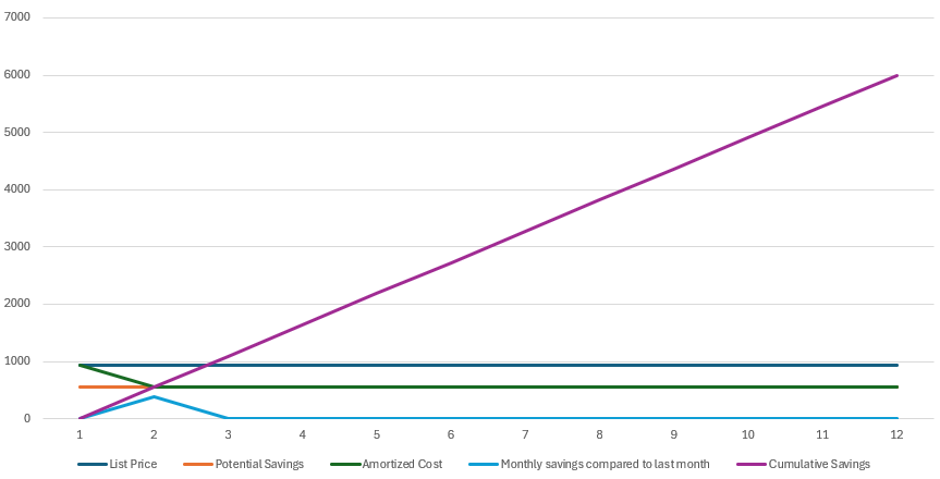
The graph lines are:

• List price = The cost of resources at Azure list price, with no commitment discounts applied.

• Potential savings = The amount you would save by applying the schedule, compared to list price with no schedule.

• Amortized cost = The price you actually paid.

• Monthly savings compared to last month = Expect a spike in month 2 as the schedule takes full effect. From month 3 onwards, savings remain consistent; there are no new savings beyond what was already achieved.

• Cumulative savings = The total savings accumulated over time, compared to taking no action.

Sample Data Behind Graph